
Evaluating investment performance based solely on returns tells an incomplete story, particularly when different portfolios carry varying levels of risk. The Sharpe ratio addresses this challenge by measuring risk-adjusted relative returns, making it one of the most widely used metrics amongst investors and analysts. Economist William F. Sharpe proposed this ratio in 1966 following his work on the capital asset pricing model (CAPM).
Generally, the higher the Sharpe ratio, the more attractive the risk-adjusted return, with values of 1 considered good, 2 even better, and anything 3 or above very good. This article explores Sharpe ratio interpretation across different asset classes, including sharpe ratio crypto applications, and examines complementary metrics such as max drawdown crypto to provide a comprehensive framework for investment decision-making.
Understanding the Sharpe Ratio Formula
Components of the Sharpe Ratio Equation
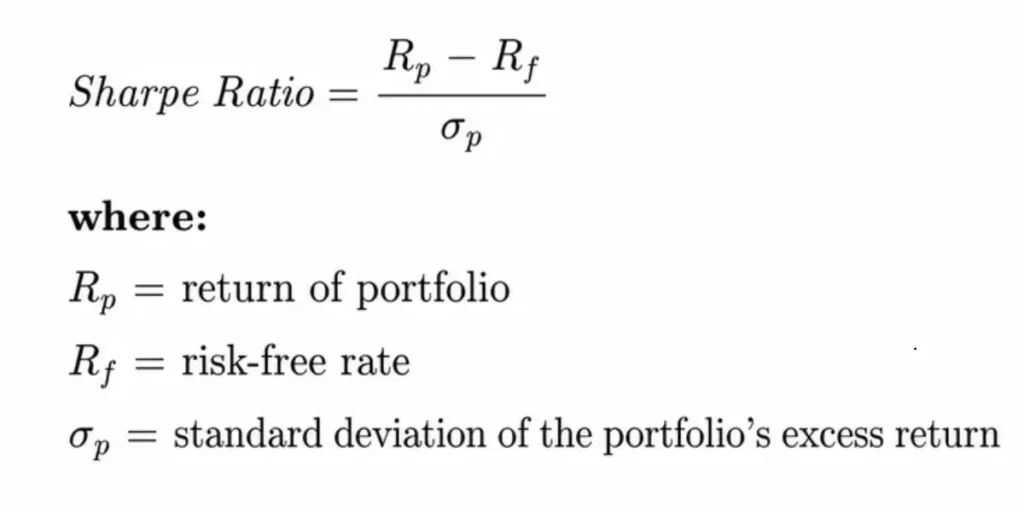
The mathematical structure behind the Sharpe ratio follows a straightforward formula: (Rp – Rf) / σp. This equation contains three distinct elements that work together to quantify risk-adjusted performance. Rp represents the expected portfolio return, essentially the gain or loss realised by an investment over a specific measurement period. Rf denotes the risk-free rate of return, typically proxied by yields on short-term government bonds such as UK gilts for GBP-denominated strategies or US Treasury bills for USD strategies. The denominator, σp, captures the standard deviation of the portfolio’s returns, serving as the proxy for total volatility.
Expected Return Minus Risk-Free Rate
The numerator isolates what investors call excess return, stripping out the return achievable without bearing any risk. If the risk-free rate sits at 4% and a portfolio returns 12%, the excess return equals 8%, representing compensation received specifically for accepting risk. This difference must remain positive, as a negative value would indicate that investing in risk-free financial instruments would have generated superior returns compared to the fund manager’s performance. In the current environment where UK base rates have settled around 3.5-4%, the risk-free rate carries meaningful impact on Sharpe ratio interpretation. This contrasts sharply with the near-zero rate environment of 2020-2021, when the risk-free component barely influenced calculations.
Standard Deviation as a Measure of Risk
Standard deviation measures total volatility by capturing both upside and downside movements in returns. A return series that fluctuates significantly produces high standard deviation, whilst one moving within a narrow range shows low standard deviation. For instance, a portfolio with an expected return of 10.0% and standard deviation of 6.0%, combined with a risk-free rate of 2.5%, yields a Sharpe ratio of 1.25x. Standard deviation treats a +3% return and a -3% return as equally risky, which represents one key limitation of the Sharpe ratio. Investors typically welcome upside surprises, yet this metric penalises them identically to negative surprises. The ratio remains the industry standard nonetheless, owing to its simplicity and universal acceptance across investment contexts.
Step-by-Step Guide to Calculate the Sharpe Ratio
Gathering Historical Return Data
Historical return data forms the foundation for Sharpe ratio calculations. Investors typically examine longer timeframes to avoid basing judgements on short-term market noise. Sources for this data include platforms offering annual returns of over 50 asset classes dating back to 1970, with some reaching 1900. Research covering the global multi-asset market portfolio from 1960 to 2017 documents a compounded real return of 4.45% with 11.2% standard deviation. The numerator calculation involves averaging return differentials across incremental periods; for instance, a 10-year ratio might average 120 monthly return differentials versus a benchmark.
Determining the Appropriate Risk-Free Rate
The risk-free rate should match the duration of projected cash flows. Most investors use the 10-year US Treasury note yield as the preferred proxy, despite longer-maturity bonds offering better duration matches, owing to limited liquidity and data availability for extended maturities. On 2 January 2024, the 1-year T-bill rate stood at 4.8%. Investors must distinguish between nominal and real risk-free rates, with the real rate calculated as (1 + Nominal Rate) ÷ (1 + Inflation Rate). The selected rate should align with whether cash flows are expressed in nominal or real terms.
Computing Portfolio Volatility
Standard deviation quantifies portfolio volatility through a specific process. First, calculate the return variance from the average return in each incremental period, square it, then sum all squared values. Subsequently, divide this sum by the number of periods and take the square root of the quotient. For annualisation purposes, multiply daily standard deviation by the square root of 252 (trading days). Monthly volatility requires multiplication by the square root of 12.
Sharpe Ratio Crypto Calculation Considerations
Cryptocurrency assets present unique challenges for sharpe ratio crypto calculations. Bitcoin’s substantial volatility requires careful interpretation of whether returns justify the risk exposure. For continuously priced crypto data, 365-day annualisation may prove more appropriate than the conventional 252-day convention used for equities.
Sharpe Ratio Interpretation and Benchmarks
Reading Sharpe Ratio Values Correctly
Positive values indicate the portfolio outperformed the risk-free rate, whilst negative readings signal underperformance against risk-free assets. When excess returns turn negative, interpretation becomes problematic, as higher volatility paradoxically produces a less negative (seemingly better) ratio. The primary takeaway remains straightforward: negative values mean the investment failed to clear even the lowest performance hurdle.
Industry Standards for Good Sharpe Ratios
Ratios above 1.0 are considered acceptable to good by investors. Values above 2.0 rate as very good, whilst those exceeding 3.0 are deemed excellent. However, most diversified indices of equities, bonds, mortgages or commodities show annualised ratios below 1.0, suggesting that figures consistently above 2.0 or 3.0 may prove unrealistic.
Comparing Your Portfolio Against Market Indices
A portfolio with a 1.0 ratio might appear lacking if most rivals achieve readings above 1.2. Accordingly, investors should compare the sharpe ratio of portfolios or funds against peers or market sectors rather than relying on absolute thresholds. Alternative investments demonstrate the highest ratios amongst asset classes, indicating superior risk-adjusted performance.
Understanding Context-Dependent Interpretations
A single number proves meaningless without context. What counts as good varies significantly by strategy: passive equity indices historically achieve 0.3 to 0.5, long/short equity hedge funds typically target 0.8 to 1.5, whilst market-neutral statistical arbitrage often reaches 1.5 to 3.0.
Using the Sharpe Ratio for Investment Decisions

Evaluating Portfolio Performance
Investment professionals apply the Sharpe ratio to determine whether portfolio returns adequately compensate for risk exposure. Ratios between 0.5 and 1.0 are considered acceptable, whilst those below 0.5 suggest insufficient compensation for risk taken. The ratio serves as the standard measure for comparing funds across different risk levels, as raw returns mislead when volatility profiles differ.
Limitations You Need to Know
Standard deviation treats upside and downside volatility equally, penalising funds with large positive surprises identically to those with negative ones. Funds with non-normal return distributions, particularly hedge funds, can artificially inflate ratios. Serial correlation tends to smooth volatility, potentially overstating the ratio by up to 65%.
Alternative Risk-Adjusted Metrics
The Sortino ratio substitutes downside deviation for standard deviation, targeting only harmful volatility. The Treynor ratio uses beta instead, measuring systematic risk for diversified portfolios. Jensen’s alpha identifies manager skill through benchmark-adjusted returns.
Max Drawdown Crypto and Complementary Measures
Maximum drawdown measures the largest peak-to-trough decline before recovery. Bitcoin’s max drawdown crypto exceeds 85% historically. The Calmar ratio divides annual return by maximum drawdown, with values above 3.0 considered strong.
Conclusion – Sharpe Ratio
The Sharpe ratio remains an essential tool for evaluating risk-adjusted performance across asset classes. By dividing excess returns by standard deviation, it provides investors with a standardised method to compare portfolios carrying different risk profiles. Values above 1.0 generally indicate acceptable performance, though context matters considerably across strategies. Equally important, investors should recognise its limitations and employ complementary metrics like Sortino ratio and maximum drawdown for comprehensive portfolio analysis. All things considered, the Sharpe ratio delivers valuable insights when applied thoughtfully alongside other risk measures.
You May Also Be Interested In: The Bitcoin 4-Year Cycle Explained: A Strategic Guide for 2026
What does a good Sharpe ratio look like for different investment strategies?
A Sharpe ratio above 1.0 is generally considered acceptable to good, whilst values above 2.0 are very good and those exceeding 3.0 are excellent. However, context matters significantly: passive equity indices historically achieve 0.3 to 0.5, long/short equity hedge funds typically target 0.8 to 1.5, and market-neutral statistical arbitrage often reaches 1.5 to 3.0. Warren Buffett’s long-term Sharpe ratio is approximately 0.75.
Why does the Sharpe ratio treat upside and downside volatility the same way?
Standard deviation, which the Sharpe ratio uses to measure risk, treats both positive and negative return movements equally. This means a +3% return and a -3% return are considered equally risky, even though investors typically welcome upside surprises. This represents one key limitation of the metric, which is why complementary measures like the Sortino ratio (which focuses only on downside deviation) are often used alongside it.
What special considerations apply when calculating the Sharpe ratio for cryptocurrencies?
Cryptocurrency assets present unique challenges due to their substantial volatility. For continuously priced crypto data, 365-day annualisation may prove more appropriate than the conventional 252-day convention used for equities. Additionally, Bitcoin’s historical maximum drawdown exceeds 85%, so it’s essential to use complementary risk metrics alongside the Sharpe ratio to fully assess crypto investment performance.